ABSTRACT

An upper-ocean vortex associated with tropical instabilities was observed during fall 1990 at 140°W in the shear region between the Pacific South Equatorial Current and the North Equatorial Counter current. The velocity and thermohaline structures of the vortex were mapped in three dimensions using hydrography, acoustic Doppler current measurements, drifters, and satellite infrared images.

The vortex translated westward at 30 cm s¹ (0.24° day¹), stationary relative to the mean flow, and less than half the 80 cm s¹ speed of contemporaneous meridional oscillations of the Equatorial Undercurrent and South Equatorial Current. The coherent flow pattern was restricted to above the thermocline. Convergence at the North Equatorial Front and divergence near the vortex center occurred in a dipole pattern similar to those predicted by various numerical models. The convergence and the anticyclonic vorticity were of the same magnitudes as the local inertial frequency, suggesting that the feature was a fully nonlinear, large Rossby number vortex, and may have been subject to centrifugal instability.

The anticyclonic flow was associated with a thermocline depression of 30 m and a deformation of the North Equatorial Front. Northward advection of cold, saline, equatorial water and southward advection of warmer, fresher, tropical water yielded the cusplike surface temperature pattern commonly associated with tropical instabilities. Equatorward heat and freshwater fluxes implied cooling and freshening from 3°N to 5°N, comparable to the annual-mean net surface heating and evaporation minus precipitation for the region.

1. Introduction

The circulations of the tropical Pacific and Atlantic Oceans are characterized by alternating zonal currents:the westward South Equatorial Current (SEC) straddling the equator, the eastward Equatorial Undercurrent (EUC) embedded within the SEC along the equator, and the eastward North Equatorial Countercurrent (NECC) to the north. The southeast trades induce upwelling as they cross the equator, forming the North Equatorial Front (NEF) between the cold equatorial tongue and warmer waters to the north. Each year in late summer to fall, when the intertropical convergence zone (ITCZ) migrates northward, the southeast trades accelerate the SEC and meridional oscillations perturbing the zonal currents are observed at periods of 15–35 days and wavelengths of 500–1500 km. The long wavelength of the oscillations of the NEF seen in satellite images of sea surface temperature (SST) led to the name “equatorial long waves,” while stability analyses of the mean currents prompted the name “tropical instability waves” (TIWs).

These oscillations were first detected in current meter records as meanderings of the Atlantic SEC (Düing et al. 1975 ) and in satellite infrared images as cusplike deformations of the Pacific NEF (Legeckis 1977 ). They appear in the tropical Pacific as meanders of the EUC and SEC, meridional deformations of the NEF, and anticyclonic vortices and sea level highs in the SEC– NECC shear. They have been observed using drifters (Hansen and Paul 1984 ; Chew and Bushnell 1990 ), current meter arrays (Lukas 1987 ; Halpern et al. 1988 ; Bryden and Brady 1989 ; Qiao and Weisberg 1995 ), velocity profilers (Leetmaa and Molinari 1984 ; Wilson and Leetmaa 1988 ; Luther and Johnson 1990 ), inverted echo sounders (Miller et al. 1985 ), moored thermistors (McPhaden 1996 ), satellite infrared images of SST (Legeckis et al. 1983 ; Legeckis 1986 ; Pullen et al. 1987 ), satellite altimeters (Perigaud 1990 ; Busalacchi et al. 1994 ), and visually from the space shuttle (Yoder et al. 1994 ). Their predicted and observed meridional eddy fluxes of heat and momentum are comparable to the fluxes associated with the annual mean circulation (Cox 1980 ; Hansen and Paul 1984 ; Philander et al. 1986 ; Philander et al. 1987 ; Semtner and Chervin 1988 ; Bryden and Brady 1989 ; Johnson and Luther 1994 ; Baturin and Niiler 1997 ).

The 1990 Tropical Instability Wave Experiment (TIWE) was designed to study the structure, kinematics, and dynamics of tropical instabilities in the Pacific Ocean. A preliminary overview of the experiment (Flament et al. 1996 ) revealed the presence of a coherent vortex moving westward in the SEC–NECC shear zone between 2°N and 7°N. Here, we study in more details the kinematics of the vortex, and describe the associated three-dimensional velocity and thermohaline structure of the upper ocean. We show that a SST cusp and a sea level high propagating westward were signatures of this coherent vortex, which appeared distinct from wavelike disturbances observed simultaneously at the equator. The similarity with instabilities modeled by the Parallel Ocean Climate Model (POCM) strengthens the observations, limited by design to one event, and suggests that our results may apply generally to SEC–NECC shear vortices.

The terms tropical instability wave (TIW) and equatorial long wave were both originally chosen to describe the smooth, linear wavelike appearance of SST cusps in the tropical Pacific (Legeckis 1977 ; Philander et al. 1985 ). The observations presented here suggest that the phenomena, collectively called TIWs in the literature, may consist of more than one distinct process. For internal consistency within this paper, we will use the term “tropical instability vortices” (TIV) to refer to the highly nonlinear SEC–NECC shear vortices, and reserve “equatorial disturbances” or “equatorial long waves” for near-equatorial oscillations of the EUC–SEC system.

The instruments, the sampling strategy, and the data are described in section 2. The measurements are integrated into a coherent representation of a translating vortex in section 3. The surface and subsurface structures of the vortex are presented in sections 4 and 5. The observations are summarized and discussed in section 6

2. Overview of the experiment

The Tropical Instability Wave Experiment included two survey cruises to the central tropical Pacific Ocean during the peak of the 1990 instability season: TIWE-1 focused on the small-scale structure of the NEF (Sawyer 1996 ), while TIWE-2 sampled the large-scale dynamic and thermohaline structure of the SEC–NECC shear region (Kennan 1997 ).

During TIWE-2, a counterclockwise rectangular survey spanning 2°–5°N, 139.25°–140.75°W was repeated by the R/V Moana Wave six times over a 20-day period (Fig. 1 ). Shipboard acoustic Doppler current profiler (ADCP) (Firing et al. 1994 ), repeated CTD casts (Trefois et al. 1993 ), and a towed undulating platform (SeaSoar) (Sawyer et al. 1994 ) measured the velocity and thermohaline fields over the upper 300 m of the ocean. Drifting buoys were deployed at the corners of the survey box and in clusters to observe smaller-scale processes. Infrared SST images were available in real time onboard the ship. Surface fluxes were measured by a fully instrumented air–sea interaction tower 10 m above water level, 2 m ahead of the bow of the ship (Flament and Sawyer 1995 ).

The data were augmented by the Tropical Atmosphere–Ocean (TAO) array of moorings spanning 2°S to 9°N at 140°W (Hayes et al. 1991 ; McPhaden 1995 ), and by an equatorial array of moored ADCPs (Weisberg et al. 1991 ; Qiao and Weisberg 1995 ). Profiling current meters (PCMs) near 2°N, 140°W provided additional measurements (C. Eriksen 1998, personal communication). All available data are shown in Fig. 1 . The timing of the deployments of the various instruments are shown in Fig. 2 , with time series of shipboard winds, currents at the equator, and temperature profiles at 5°N, 140°W. The observations, made from 16 November to 6 December 1990 (days 320–340), coincided with a deepening of the thermocline at 5°N and a meridional oscillation of the SEC at the equator.

a. Lagrangian drifting buoys

The drifters were standard World Ocean Circulation Experiment Surface Velocity Project (WOCE-SVP) buoys, with a 7.5-m holey sock drogue and a surface temperature sensor (Niiler et al. 1995 ). The nominal depth of the drogues was 15 m. Strong vertical shear may decrease this depth, especially in the EUC. The drifters were tracked by ARGOS five to eight times daily, and the positions were objectively interpolated onto regular 3-h time intervals (Hansen and Poulain 1996 ).

The drifters were deployed in clusters near 3.25°N, 140°W on day 323 (seven drifters) and near 1.8°N, 141°W on day 336 (eight drifters). Additional drifters were deployed individually around the survey box. Most of the drifters moved westward in trajectories resembling cycloids, similar to those observed by Hansen and Paul (1984) and Chew and Bushnell (1990) .

The first two drifters, deployed at 3.5°N on day 322, looped rapidly clockwise while drifting westward with the SEC (Fig. 3a ). The next two, deployed near 2°N on day 322, moved slowly northward at 18 cm s¹ and westward at 59 cm s¹ with the SEC (Fig. 3b ). They reached 4.5°N on day 345 before meandering eastward in the NECC.

On day 323, seven drifters were deployed as a cluster centered at 3.7°N, 140.3°W with a spacing of about 10 km, to measure velocity gradients across the surface temperature front (Fig. 3c ). All proceeded rapidly northward. Upon reaching 6°N, one was entrained into the NECC, while the others continued the cycloidal motion.

Of the remaining drifters deployed individually, three more followed looping trajectories. The others showed some signs of looping, but spent most of their time in either the SEC or NECC (Fig. 3d ).

On day 335, a second cluster of eight drifters was deployed in the SEC. They drifted westward and then northward, until the end of the experiment (Fig. 3e ).

Of the drifters deployed, one crossed the equator at 60 cm s¹ (not shown). For the others, looping simultaneously stopped around day 350. This day was also the end of the last pulse of northward flow observed at the equator (Qiao and Weisberg 1995 ) (Fig. 2 ). Thus, the drifters sampled the flow between the SEC and NECC near the end of the instability season.

b. Acoustic Doppler current profiler

The shipboard ADCP measured velocity of the upper 300 m along the ship track (Firing et al. 1994 ). The velocity at 22 m is shown in Fig. 4 for each of the six circuits. At the start of the survey, there was little flow at 5°N (Fig. 4a ), but the SEC had intensified to 1 m s¹ by the time the ship was at the southeast corner of the box. Northward flow of about 1 m s¹ was found along 5°N when the circuit closed. For each subsequent circuit, the flow was dominated by the westward SEC, but a progression from northward to southward flow is seen in Figs. 4b–d .

3. A translating vortex

a. Determining the translation speed

The drifters seeded in the cold water cusp followed cycloidal trajectories, which may be expressed in general as

x_i(t) = A_isin(2t/T_L)+B_icos(2t/T_L)+C_it+D_i (i = 1, 2), (1)

1

1

1

The looping trajectories indicate the westward propagation at 30 cm s¹ of a disturbance in the SEC– NECC shear. Independent estimates of the propagation speed are obtained by (i) tracking the cusplike disturbance of the NEF in satellite images and (ii) calculating the lags between velocity variations along the meridional survey legs.

Due to cloud cover, the SST front was only visible in a few images. Figure 8 shows weekly composites of Pathfinder images for four time periods spanning the experiment. In each image, the cold tongue extends along the equator, with warmer water to the north. The longitude of the leading front of the SST cusp is identified within an error bar in each image. The propagation speed over six weeks varied from 23 to 53 cm s¹. This large range may be due to smearing of the front in the weekly composites. However, the speed estimated while the drifters were looping is 23 ± 9 cm s¹, consistent with the 30 cm s¹ obtained from the cycloid fits.

The propagation speed can also be estimated from shipboard ADCP measurements along the western (140.75°W) and eastern (139.25°W) survey legs (Fig. 4 ). The data along each leg were linearly interpolated in time (Fig. 9a ). For the decreasing phase of meridional velocity, the median lag between the two legs was estimated for each ¼° latitudinal bin between 3°N and 4.75°N. The propagation speeds ranged from 35 to 70 cm s¹ (Fig. 9b ).

The various estimates of the propagation speed are given in Fig. 10 , along with estimates from minimum mapping errors and longitude–speed correlations, discussed below. They are consistent with the interpretation that the drifters resided on closed streamlines in a frame of reference translating with the disturbance, as argued below. The speed obtained from the Lagrangian drifters is the most robust, and lies within the error bars of the other estimates.

b. Closed streamlines

Did the looping trajectories result from a westward propagating wave or from a translating vortex? In the former case, drifters would not move on average with the disturbance, while in the latter they would follow closed streamlines in the frame of reference translating at C_i. To distinguish between these two situations requires independent Lagrangian and Eulerian estimates of the translation speed.

The average zonal displacement speed c_d of a drifter, equivalent to C₁ in (1), and the zonal translation speed of the disturbance c_t are

An independent measure of the Eulerian period T_E is obtained from the TAO thermistor chain at 5°N, 140°W. The passage of the central high pressure of the vortex was marked by minima in the temperature at 180-m depth around days 310 and 340 (Fig. 2d ), thus T_E = 30 ± 5 days. For T_L = 20 days and c_d = 30 cm s¹, the only possible open streamline solutions for c_t would be 11 to 13 cm s¹ or +40 to +120 cm s¹, in contradiction with the estimates for c_d ranging from 23 to 70 cm s¹ (Fig. 10 ). Therefore, the drifters must have resided on closed streamlines, being entrained in a vortex translating to the west at c = c_d = c_t = 30 ± 1 cm s¹.

c. Mapping the vortex

The vortex was mapped in the translating frame of reference defined as

x = x ct,y = y, (2)

1

In this case, the transformation offers a synoptic view of the vortex, from data widely separated in space and time. The remapped velocities are shown in Fig. 11 . The longitude scale corresponds to 0000 UTC 25 November. In the translating frame, the drifter loops close on themselves while the ship and the moorings appear to progress eastward. The SEC is weaker and the NECC stronger by 30 cm s¹. Velocities collocated in the translating frame, but observed at varying times and positions in the fixed frame, agree well north of 2°N, indicating that drifter trajectories and streamlines coincided, thus that the relative flow was approximately steady. Along 4.25°N, the relative zonal flow is very small: the vortex in the SEC–NECC shear was stationary with respect to the mean zonal flow. In other words, the westward translation of the vortex was entirely advective.

However, collocated velocity vectors from the moorings near the equator do not agree, indicating that fluctuations there translated at a different speed. The phase speed of the equatorial signal, determined by cross-correlations between pairs of moorings, was 80 cm s¹— more than twice the speed of the vortex. Therefore, the transformation into the 30 cm s¹ translating frame is only valid north of 2°N. Viewed instead in the frame translating at 80 cm s¹, the mooring data agree well (Fig. 11 ), but there is no vortex pattern: the disturbance is a meandering of the SEC, as described previously (Düing et al. 1975 ; Halpern et al. 1988 ). In contrast to the vortex, there is an eastward relative zonal flow along the equator: the oscillations propagated westward relative to the mean zonal flow.

The transformed data north of 2°N were interpolated onto a regular grid with a spacing of ¼°, using a median filter of radius 75 km centered on each grid point (see the appendix). The median is insensitive to outliers while preserving sharp gradients.

The success of the interpolation can be assessed by calculating the velocity mapping error (see the appendix). It should be minimum in the frame of reference translating with the vortex: in other frames, the relative flow would not be steady and the mapping error would be larger. The longitudinally averaged error is contoured as a function of translation speed c and latitude in Fig. 12 . North of 1.5°N, the error is minimum for speeds ranging from 29 to 39 cm s¹, in agreement with the interpretation of a coherent vortex. Near the equator, the error is minimal for 80 cm s¹, in agreement with the phase speed inferred from the moorings. This confirms that the kinematics near the equator and in the shear between the SEC and the NECC were distinct, with an abrupt transition between them.

The correlation between meridional velocity and transformed longitude x as a function of translation speed c provides another assessment of the adequacy of the translating frame to map the vortex. Figure 13a (solid line) shows the correlation computed using only the looping drifters; it is most significant around 26 cm s¹. Computations using all drifters, and all data including moorings and ADCP, fall in the range of 20 to 30 cm s¹. However, for correlations computed using ADCP data only, there is a striking contrast below and above the 120-m deep thermocline (Fig. 13b ): in the upper layer, the correlation is significant for westward translations; below the thermocline, the correlation remains barely different from zero at all translation speeds. Therefore, the mapping of the fields in the translating frame of reference is only meaningful above the thermocline.

4. The surface flow

a. Temperature and salinity advection

The gridded velocity field, based on all the available velocity data, is shown in Fig. 14 , superposed on the (properly translated) SST image from 16 November. The cusplike pattern typical of tropical instabilities is seen, distorting the NEF. The velocity field reveals an anticyclonic vortex with speeds approaching 1 m s¹. The cold water cusp coincides with northward flow along the leading edge of the vortex. Although the image is instantaneous while the velocity map was sampled over 20 days, the association of the cold cusp with the vortex is striking. Northeastward flow also exists to the northeast of the map, sampled by a single drifter and by the last ADCP track, possibly indicating a subsequent vortex in a train of coherent structures.

The errors of the velocity components were estimated as described in the appendix. Most of the velocity field is known to ±5 cm s¹, or 10% (Fig. 14b ). Larger errors near 138°W and north of 5°N probably result from temporal changes in the flow. Nevertheless, the vortex remained steady to lowest order. Gridded without the drifters, the flow is similar (Fig. 15a ), but errors are larger, 15%, since there are fewer degrees of freedom (Fig. 15b ). Subsequently, the analysis will be limited to the velocity field obtained from this subset, to avoid mixing data from drifters sampling at 15-m depth, with the shallowest depth of the ADCP at 20 m. The three-dimensional view will also be simplified by having constant sample sizes as a function of depth.

The gridded temperature field (from drifters, underway thermograph, and CTD casts, Fig. 16a ) shows the same cold water cusp as the Advanced Very High Resolution Radiometer (AVHRR) image, with a comparable temperature front (>1°C). The salinity pattern is analogous, with high salinity water (35 psu) flowing northward from the southwest, and low salinity water (34.5 psu) flowing southward from the northeast (Fig. 16b ). This suggests that TIVs induce a net salt flux, just as they transport heat (Hansen and Paul 1984 ).

The density at the surface mirrored the patterns of temperature and salinity, with dense water flowing northward and lighter water flowing southward (Fig. 16c ). At depth, however, the density field reflected a central high pressure associated with the anticyclonic flow of the vortex. The = 24.7 isopycnal lay within the thermocline over the entire study region; its depth is mapped in Fig. 16d . The zonal changes in upper-layer thickness is 30 m at the latitude of the center. The pycnocline density step being 4 kg m³ or 0.4%, the implied sea surface height signature is about 12 cm, consistent with previous observations from inverted echo sounders and satellite altimeters (Miller et al. 1985 ; Perigaud 1990 ; Busalacchi et al. 1994 ).

b. Eddy heat and salt fluxes

The mean eddy fluxes of heat and salt can be estimated by averaging the gridded data zonally, temporal averaging at a fixed point being equivalent to zonal averaging in the translating frame. This implicitly assumes that one complete, and representative, wavelength of a train of vortices was sampled. Figure 17 shows the zonally averaged eddy heat flux and advection in the zonal and meridional directions. Error bars were estimated using stochastic simulations, with eight degrees of freedom in the zonal average.

The vortex transported heat equatorward and eastward, in agreement with the observations of Hansen and Paul (1984) and Baturin and Niiler (1997) (Figs. 17a,b ). However, the heat flux reached only 0.3 × 10⁶ W m², less than the 0.4 to 0.8 (×10⁶ W m²) found in studies based solely on drifters. By recalculating the flux using drifters only (curves with bullets in Fig. 17 ), the magnitude of the meridional eddy heat flux increases 33%, to 0.4 × 10⁶ W m².

The method of calculating fluxes has therefore an impact on the results. Drifters do not sample the velocity field homogeneously in the presence of TIVs; they tend to either travel along closed streamlines within the vortex, or escape in the SEC or NECC, but do not sample well between vortices or near their centers. Consequently, they yield estimates biased by the large heat flux across the perturbed NEF. Fluxes computed instead from the gridded fields over the entire extent of a vortex are not biased by the inhomogeneous sampling. Previous heat flux estimates may have been too large by 50% to 250%.

Using zonal averaging, a heat equation is

Between 2°N and 5°N, the surface layer gains heat from the eddy zonal flow and loses heat from the meridional flow; there is a net loss of 0.5 W m³ north of 2.5°N (Figs. 17e–g ). Again, the estimates based solely on drifters agree with Baturin and Niiler (1997) .

The net air–sea heat flux measured by the shipboard meteorological sensors is shown zonally averaged in Fig. 17c ; it ranged from 50 to 150 W m², larger than the 25 W m² annual mean (Weare et al. 1981 ) (the errors were estimated without the shortwave radiation term, exhibiting a large diurnal cycle but measured accurately). The depth over which the air–sea heat flux acts is needed to compare it with the eddy heat flux. The mixing layer and thermocline depths are presumably shallow and deep bounds on this depth; in the Tropics, wind forcing may easily deepen the mixing layer down to the thermocline, while surface heating may quickly restratify the water column (the deeper bound may be more appropriate since the surface layer is often at constant temperature down to the thermocline). The zonally averaged mixed layer and thermocline depths are shown in Fig. 17d ; they range from 40 to 150 m. The air–sea heat flux divergence then ranges from 0.5–1 W m³. Between 3°N and 5°N, it opposes significantly the 0.5 W m³ eddy heat flux convergence.

The vortex transported freshwater equatorward and saline water northward; the zonal flux was insignificant (Figs. 18a,b ). Between 3°N and 5°N, there is a net freshening of 0.2 × 10³ g (m³s¹) (Figs. 18e–g ).

Again, it is useful to compare this to the net air–sea moisture flux. The moisture flux was estimated as evaporation minus precipitation (Fig. 18c ). Evaporation dominated at 0.06 to 0.08 g m² s¹, or 6 to 8 mm day¹. This may not be representative of the mean conditions since the ITCZ borders to the north and exhibits a seasonnal migration. Other estimates of the mean annual rainfall and evaporation minus precipitation for this region range from 2 to 6 mm day¹ and 3 to +3 mm day¹, respectively (Janowiak and Arkin 1991 ; Jourdan et al. 1997 ). During the instability season when the ITCZ is farthest north, evaporation should dominate south of 8°N, as we observed.

Averaged over the thermocline depth, the observed surface flux corresponded to a net freshwater loss of 0.5–2 mg m³ s¹, while the net effect of the annual mean ranges from 1 to 1 mg m³ s¹. The vortex caused a net freshening of 0.2 mg m³. Consequently, the freshwater flux induced by TIVs may represent 20%–100% of the net freshwater balance from 3° to 5°N.

c. Horizontal divergence and vorticity

Horizontal divergence and relative vorticity were estimated from the gridded ADCP velocity field by central differencing. The standard errors were calculated using stochastic simulations (see the appendix). Both fields were normalized by the inertial frequency f at 4°N (f = 10⁵ s¹), while the error fields are represented as signal to noise ratios—e absolute value of the divergence, or vorticity, divided by its standard error.

Divergence reaches f around 3.5°N, 142°W, while divergence near +f occurs to the east (Fig. 15c ). The pattern is significantly different from zero; the core of convergence is almost three standard errors from zero (Fig. 15d ). Divergence over the remainder of the vortex is not significant.

The divergence estimated with drifting buoy data included is not shown. It gives a weaker maximum convergence (f/2), without changing the overall pattern (Flament et al. 1996 ; Kennan 1997 ). This may be due to the surface-constrained drifters providing a biased sampling of the velocity field: they tend to align along convergent fronts and avoid divergent regions, sampling the flow inhomogeneously. A similar sampling bias was encountered when estimating the heat flux.

The relative vorticity (Fig. 15c ) was negative (anticyclonic) over much of the vortex, reaching f at 4°N, 141°W and 4°N, 139.5°W near the center. A ridge of positive (cyclonic) vorticity greater than f/2 circles the western flank of the vortex. It is apparently associated with the perturbed NEF. Again, this pattern is significant (Fig. 15e ). The intense relative vorticity field indicates that the flow was highly nonlinear, with a large Rossby number, of the order of Ro = 1.

Increased vorticity and convergence near the front were also directly measured using a cluster of seven drifters, deployed with a mean separation of 10 km on the southeast side of the front. The cluster progressed northwestward while shrinking in area (Fig. 19 ). After collapsing onto the front, the drifters continued to move around the vortex more or less along the same streamline (Fig. 3c ). The average cluster temperature increased as it approached the front (Fig. 20a ).

Over a region the size of the cluster, the velocity field may be expressed as a first-order Taylor expansion around the center (Flament and Armi 2000 ):

On 30 November, a second cluster of eight drifters with a mean separation of 10 km was deployed farther south near 2°N, 139°W (141°W in the absolute frame of Fig. 3e ). In contrast to the first cluster, it moved westward for several days without deforming; the divergence was barely significant and uniform at 0.1 f, in agreement with the large-scale gridded field.

The velocity gradient near the front exhibited a fivefold increase compared to the gridded field, which smoothes out and thus underestimates sharp gradients. Similar scaling of the deformation field with the horizontal length scale has been observed at other oceanic fronts (Flament and Armi 2000 ).

Figure 21a shows velocity and temperature of the uppermost level (0–25 m) over the region 1°S–9°N, 170–115°W on 21 November, five days after the satellite image of the vortex (Fig. 14 ). Three well-developed vortices are present at intervals of about 10°, with maximum speeds of about 1 m s¹ along the front. The relationship between the anticyclonic TIVs and cusplike disturbances of the NEF is confirmed by the modeled temperature field.

Each TIV has a dipole of intense convergence and divergence of 0.5f along its western edge, aligned with the cold cusps. The relative vorticity is also consistent with the observations, approaching f near the center of the vortex, with a ridge of positive (cyclonic) vorticity. The correspondence between the observations and the simulations is striking, and in agreement with other models. The POCM strengthens the observations of the distribution of divergence and relative vorticity, suggesting that they may be general features of TIVs.

1

1

The Ekman pumping velocity (Fig. 22c ) shows a deepening of the thermocline near 3°N, 138°W at over 20 m day¹, and a shoaling to the south. The vertical velocity obtained by integrating the divergence down to 125-m depth similarly shows downwelling at 20 m day¹ near 3°N, 138°W and upwelling to the south (Fig. 22d ). This suggests that this pattern is not real and results from temporal rather than spatial variations of the Ekman transport. The azimuthal asymmetry of the vortex high pressure center (Fig. 16d ) may also be spurious. Although temporal changes of the vortex are projected into spatial patterns in the translating frame, the steadiness assumption appears to break down only in this relatively small area, away from the NEF, where the observed pattern of convergence and divergence is real.

5. The three-dimensional structure

Velocity, temperature, and salinity were also gridded as a function of depth for 10-dbar depth intervals from 20 dbar to the thermocline. Vertical sections zonally through the vortex center (along 4.25°N, Fig. 23 ) and meridionally through the frontal convergence (along 140°W, Fig. 24 ) will now be presented.

3

1

The meridional section of zonal velocity along 142°W is shown in Fig. 24a . The SEC extends down to the thermocline, with speeds larger than 25 cm s¹. At 3°N, the SEC approaches 1 m s¹ above 25 dbar. Although the survey did not extend north of 5.25°N, current meter moorings at 7°N indicated a swift eastward NECC greater than 50 cm s¹, down to 100 m.

To the lowest order, these vertical sections reveal a strong anticyclonic flow, relatively coherent down to the thermocline. To the next order, they reveal east–west asymmetry with the core of maximum speed occurring shallower in the northward branch than in the southward one.

b. Temperature and salinity

The zonal section of temperature shows a deepening of the thermocline near the center of the anticyclonic vortex (Fig. 23b ). There is also an upward bowing of isotherms associated with the cold northward flow. The leading edge of the NEF extends past 80-m depth at 142°W. In the meridional section, the subduction of cold water at the front is seen near 4°N (Fig. 24b ). The zonal section of salinity shows freshwater flowing southward at the surface and saline water flowing northward in the cold cusp. The presence of salinities greater than 35 psu is striking in both northward and southward flows below 100 m (Fig. 23c ). This water is seen as far north as 5°N (Fig. 24c ), its presence in the return flow along 137.5°W suggests that it circuits the entire vortex. It was also observed in high resolution surveys of the front (Sawyer 1996 ).

Water of salinity greater than 35 psu is found in the South Pacific, with most of the exchange believed to occur in the western Pacific (Tsuchiya 1991 ; Bingham and Lukas 1994 ). The climatological maps of Tsuchiya (1968) show the 35 psu salinity contour occurring on the equator across most of the Pacific. At 160°W, the Hawaii–Tahiti shuttle data show the 35 psu salinity contour reaching 2°N in the upper layer (Wyrtki and Kilonsky 1984 ).

Climatological maps, however, cannot resolve the signal of tropical instabilities. It is possible that equatorial disturbances may assist the mean meridional circulation in transporting saline water across the equator. Our data indicates that this transport may be accomplished farther north by the instability vortices. This scenario is supported by the meridional section along 150°W of Montgomery and Stroup (1962) . Water with salinity greater than 35 psu reached almost 4°N, with a seemingly detached pocket of high salinity water found at 6°N (their Fig. 4 ). Their observations were made during the instability season, and are consistent with the interpretation that the high salinity water circuits the vortex.

1

1

Vertical velocities associated with TIVs appear an order of magnitude smaller O(2–5 m day¹) than this in numerical simulations (Philander et al. 1986 ; Harrison 1996 ), but an order of magnitude larger O(500 m day¹) in direct observations of the equatorial front (Johnson 1996 ; Sawyer 1996 ). The scale of the estimates clearly affects the results. Here, gridding the fields smeared out the intense signals associated with the front, which were better sampled by the cluster of drifters, yielding a convergence of 5f in agreement with other direct observations. Meanwhile, eddy-resolving models do not fully resolve fronts.

6. Summary and discussion

We observed the kinematic and thermohaline structure of a tropical instability vortex from November to December 1990 near 140°W in the Pacific Ocean. The cycloidal motion of drifters revealed an anticyclonic vortex translating westward at 30 cm s¹ (0.24° day¹) in the SEC–NECC shear. Independent estimates confirmed this speed. A translating frame of reference was meaningful to map the vortex above the thermocline and north of 2°N. The period of the associated high pressure oscillation observed from moored thermistors was 30–35 days, in agreement with previous observations (McPhaden 1996 ).

The vortex was quasi-steady, nonlinear and contained closed streamlines. There was no relative zonal flow at the latitude of the center. The perturbation did not propagate as a wave and its translation was entirely advective. The descriptor “instability wave,” suggestive of oscillations propagating due to a restoring force along the unstable shear of the zonal SEC–NECC, is thus not relevant here. For this reason, we abandoned it in favor of tropical instability vortices (TIVs) and SEC–NECC shear vortices to describe such coherent structures appearing in trains north of the equator. They are reminiscent of coherent structures observed in the laboratory in an unstable shear flow trapped within a critical layer (Lindzen 1988 ).

On the contrary, meridional oscillations of the EUC and SEC between 1°S and 1°N propagated westward at 80 cm s¹—more than twice faster than the vortex— indicating that distinct tropical instability phenomena may exist at different latitudes. The equatorial disturbance did not appear as a coherent vortical structure advected by the mean zonal flow, even though finite amplitude equatorial wave modes may have closed streamlines (Boyd 1980 ). Observations thus suggest the existence of finite amplitude waves propagating relative to the EUC–SEC shear near the equator, adequately termed equatorial long waves.

The velocity, temperature, and salinity observations were mapped in three dimensions into a frame of reference translating with the vortex. There, the flow was nearly steady, apart from a wind event which projected temporal variations into spatial gradients in the southeastern part of the vortex, where vertical velocities were attributed to aliased Ekman pumping.

The anticyclonic flow corresponded to a central high pressure and a northward cusp-shaped deformation to the NEF, in agreement with previous observations reviewed in the introduction. This relationship is consistent with shear vortices simulated by the POCM. Our results confirm that sea level highs and cold water cusps traversing the tropical Pacific with wavelengths of 500– 1500 km and periods of 25–35 days are the expressions of coherent structures, of which the vortex presented here is one example.

The magnitudes of divergence and relative vorticity, calculated from the gridded fields, both reached the inertial frequency so that the Rossby number of the vortex was Ro = 1. A dipole of convergence along the leading front of the cold water cusp, and divergence near the center of the vortex, resembled predictions by various numerical models including the eddy-resolving POCM. Relative vorticity near the center nearly exactly balanced planetary vorticity, suggesting that centrifugal instability may have acted to limit further growth or intensification of the vortex (Rayleigh 1916 ; Kloosterziel and van Heijst 1991 ; Carnevale et al. 1997 ).

The estimated convergence and relative vorticity at the leading front of the cold water cusp increased with increasing sampling resolution. While the fields gridded with a 75 km low-pass filter gave a convergence rate of f and a relative vorticity of f/2, direct measurements of the deformation of a drifter cluster at 10-km resolution yielded convergence rate and relative vorticity 5–10 times larger, of order 5f. This scaling of the velocity gradients is reminiscent of that observed near other oceanic fronts (Flament and Armi 2000 ).

The vortex entrained cold, saline water from the south and warmer, fresher water from the north, inducing net equatorward heat and freshwater fluxes of approximately 0.3 × 10⁶ W m² and 10 to 20 g m² s¹. The observed equatorward heat flux was half that computed solely from drifting buoy data, which may be biased by inhomogenous sampling. The observed equatorward freshwater flux suggests that TIVs contribute to the freshwater balance between the equator and the intertropical convergence zone. The flux divergences between 2°N and 5°N imply net cooling and freshening of about 25 W m² and 0.01 g (m²s)¹ over a mixed layer 50 m deep.

To synthesize the results of this study, we present perspective views of the three-dimensional flow and thermohaline structure of the vortex (Figs. 25 and 26 ). These views show the anticyclonic flow with the cold water cusp and depressed thermocline; northward advection of cold, saline water and southward advection of warmer, fresher water at the surface; recirculating saline water at depth; convergence along the perturbed NEF; and upwelling near the vortex center. The tropical instability was a coherent vortex in the SEC–NECC shear. It was highly nonlinear, kinematically distinct from equatorial long waves, and induced significant equatorward heat and freshwater fluxes. In a subsequent paper, we will present the dynamics and energetics of this tropical instability vortex.

Acknowledgments. We thank Capt. R. Hayes and the crew of the R/V Moana Wave for their excellent support. F. Bahr, K. Constantine, J. Firing, D. Gravatt, W. Hervig, T. Lanagan, W. Ostrom, H. Ramm, J. Ranada, K. Sanborn, M. Sawyer, K. Shultis, J. Schmitt, J. Snyder, C. Trefois, T. Young, and W. Zhou helped prepare the instruments, conduct the operations at sea, and process the data. We thank R. Knox and P. Niiler for their contributions to the cruise, and for many discussions during the analysis and interpretation of the data. J. Luyten let us use the SeaSoar from Woods Hole Oceanographic Institution. The sampling of the vortex would have been difficult without a direct HRPT receiving station installed on board by SeaSpace, Inc. Data were provided by: R. Weisberg, University of South Florida (equatorial mooring array); NOAA–PMEL TAO Project Office, M. McPhaden, Director (TAO mooring); JPL PO.DAAC (weekly MCSST composites); R. Tokmakian, A. Semtner, and B. Chervin, Naval Postgraduate School (POCM simulations); and C. Eriksen, University of Washington (2°N mooring). The plotting package gri by D. Kelley was used for Figs. 1–24 , 27 . This work was funded by the United States National Science Foundation (Grants OCE-8811430, OCE-8818732, OCE-8918604, OCE-9117078, and OCE-9633713), and by the State of Hawai’i. S. K. thanks P. Niiler for postdoctoral support at Scripps Institution of Oceanography.

u^i,j = med[^l]^i,j = med[^l],

For the various data to have equivalent weights, their spatial resolutions in the translating frame ought to be similar. The drifter positions were sampled at 3-h intervals, the ADCP at 5 min, the TAO moorings daily, and the PCMs at 4 h. The average speed of the ship was 5 m s¹, the drifters moved at 20–60 cm s¹, and the “speed” of the moorings in the translating frame was 30 cm s¹. The resolution of the drifters and PCM moorings is thus comparable at 4–5 km, while that of the ADCP and TAO moorings is 1.5 and 26 km, respectively. Consequently, the weight of the ADCP was reduced by a factor 3 (decimated to 15 min) and that of the TAO data was increased by a factor 6 (interpolated to 4 h). For the coarser (25-km spacing) hydrographic data, the TAO data was left on its daily interval.

The errors of the gridded fields are related to the variance of collocated data in the translating frame since, ideally, perfectly sampled steady fields would yield exact agreement among collocated data points. The errors depend also on the number of degrees of freedom (DOF) entering the estimate of each grid point. To estimate the DOF, the decorrelation timescale of each data type (ADCP, drifters, and moorings) was determined for each variable (zonal and meridional velocity, temperature, salinity), as the integral timescale of the relevant autocorrelation functions (

The integral timescale for drifting buoy and ADCP variables is about 2 days. Each data record was thus divided into segments with length equal to 2 days, and the number of records entering each gridpoint calculation was taken as the DOF. Mooring data was assumed to present only 1 DOF. The standard errors were taken as the square root of the variance divided by the DOF. Thus, standard errors and covariances at each gridpoint were calculated as

Central differencing was used to calculate gradients (first differences were employed at the boundaries). For example, divergence is

Errors of divergence and vorticity were estimated using stochastic (Monte Carlo) calculations. Each trial velocity component was sampled from a random distribution, p(U^i,j_q) and p(V^i,j_q), where U^i,j_q and V^i,j_q are random variables over the space ranged by q with means given by the gridpoint estimates (u^i,j and ^i,j) and standard deviations equivalent to the local standard errors (^i,j_u and ^i,j); that is,

The standard errors were then estimated as the standard deviations of M = 1000 stochastic trials:

Standard propagation of errors formulae gave similar results, but all errors in this paper were obtained using the stochastic technique.

Click on thumbnail for full-sized image.

Fig. 1. Available data from 11 Nov to 11 Dec 1990 (days 315– 345). Legend: drifter deployments (with their initial velocity, arrows);ship tracks—SeaSoar and 20-km-spaced CTD stations (solid lines), and mooring locations (circles: TAO thermistors, filled: with current meters; diamonds: upward-looking ADCP current meters; triangles: profiling current meters).

Click on thumbnail for full-sized image.

Fig. 2. Time series showing (a) the deployments of various instruments; for AVHRR and POCM the asterisks denote the synoptic pictures and for AVHRR the line bars indicate the weekly composites (the 31 Oct composite is off scale), (b) zonal (u) and meridional () wind speeds measured from the R/V Moana Wave, (c) meridional velocity components at 142°W (solid) and 138°W (dashed) on the equator, and (d) temperature from the thermistors on the TAO mooring at 5°N, 140°W and at depths 0, 20, 40, 60, 80, 100, 120, 140, 180, 300 m (bottom panel).

Click on thumbnail for full-sized image.

Fig. 3. Fifteen of the 25 drifter tracks, grouped by deployment dates and similar patterns. The heavy portions of the trajectories denote the period of the experiment. Deployment dates and days that cycloidal motion ceased are marked (day 323: 19 Nov 1990).

Click on thumbnail for full-sized image.

Fig. 4. Velocity at 22 m measured by shipboard ADCP during days (a) 320–324 (16–20 Nov), (b) 324–327 (20–23 Nov), (c) 327–331 (23–27 Nov), (d) 331–334 (27–30 Nov), (e) 334–337 (30 Nov–3 Dec), and (f) 337–340 (3–6 Dec 1990). Each survey of the rectangular area proceeds counterclockwise from the top left as indicated by insets.

Click on thumbnail for full-sized image.

Fig. 5. SST for the region 2°S–7°N, 146°–130°W at 16 Nov 1990 2319 UTC estimated from NOAA-11 AVHRR. The counterclockwise survey centered at 3.5°N, 140°W is shown. Cloudy pixels were interpolated by the median of the surrounding clear pixels in 5 × 5 boxes.

Click on thumbnail for full-sized image.

Fig. 6. Linear fit (solid line) of a constant translation speed and a single harmonic to the trajectory of a looping drifter (dashed line) (a) in the fixed frame and (b) in the translating frame of reference. In (b) 140°W corresponds to the longitude on day 329 (25 Nov) at 0000 UTC.

Click on thumbnail for full-sized image.

Fig. 7. Histograms of (a) zonal and (b) meridional translation speeds from least squares fits to the eight looping trajectories.

Click on thumbnail for full-sized image.

Fig. 8. Weekly composites of SST from AVHRR for four time periods: (a) 28 Oct–3 Nov, (b) 18–24 Nov, (c) 25 Nov–1 Dec, and (d) 9–15 Dec. White indicates cloud cover. The leading edge of the SST cusp is identified within an error bar in each composite.

Click on thumbnail for full-sized image.

Fig. 9. (a) ADCP time series of meridional velocity for the latitude bin 4°–4.25°N at 140.75°W (solid line) and 139.2°W (dashed). (b) Histogram of phase speeds determined from the lags between the time series for each ¼° latitude bins from 3° to 4.75°N.

Click on thumbnail for full-sized image.

Fig. 10. Various estimates of the translation speed. (Left) observational periods; (right) speeds and error bars for each of the following methods: cycloid regressions, SST front tracking, lags of velocity between meridional legs, velocity vs longitude correlations, and minimum velocity mapping error (see text).

Click on thumbnail for full-sized image.

Fig. 11. Velocity from shipboard ADCP and moored current meters viewed in a frame of reference translating westward with the vortex at 30 cm s¹. The trajectories of the drifters are shown dotted every 3 hours. The lower panel shows the mooring data in another frame of reference, translating westward with the equatorial disturbance at 80 cm s¹. The longitude scale corresponds to 0000 UTC 25 Nov.

Click on thumbnail for full-sized image.

Fig. 12. Velocity mapping error (in cm s¹) contoured as a function of latitude and translation speed of the frame of reference (contouring interval is 1 cm s¹ up to 10 cm s¹ and 5 cm s¹ above).

Click on thumbnail for full-sized image.

Fig. 13. Correlation between meridional velocity and longitude as a function of translation speed for (a) looping drifters (solid line), all drifters (dashed), all drifters and ADCP (dash-dotted), and (b) ADCP data above (solid) and below (dashed) the thermocline (120 m). Shading indicates one standard error from stochastic simulations.

Click on thumbnail for full-sized image.

Fig. 14. (a) Velocity in the translating frame gridded at ¼° resolution, superposed on the SST image from 2319 UTC 16 Nov 1990 (white arrows are for clarity only). (b) Standard error ellipses for velocity.

Click on thumbnail for full-sized image.

Fig. 15. Velocity, divergence (·u), and relative vorticity ( × u) estimated from ADCP data only, with their associated errors (right panels). Divergence and vorticity are normalized by f = 1 × 10⁵ s¹ at 4°N, and are contoured at 1-f intervals. Standard errors are presented as ellipses for velocity, and as signal-to-noise ratios (s/n) contoured at 0.5 intervals for divergence and vorticity.

Click on thumbnail for full-sized image.

Fig. 16. Surface maps of (a) temperature (C), (b) salinity, (c) potential density, and (d) depth of the = 24.7 kg m³ isopycnal (m).

Click on thumbnail for full-sized image.

Fig. 17. Meridional profiles of horizontal eddy heat fluxes and heat flux convergences at the surface. Heat fluxes (W m²): (a) ₀C_P (b) ₀C_P, and (c) net air–sea heat flux. (d) Zonally averaged thermocline (solid) and mixed layer (dashed) depth; and, heat flux convergence (W m³): (e) ₀C_P , (f) ₀C_P, (g) ₀C_P·, and (h) air–sea heat flux convergence estimated for the thermocline (solid) and mixed layer (dashed) depths. Dashed curves in (a–c) and (e–g) represent standard error intervals. Curves with bullets represent identical calculations, but derived from drifter data only.

Click on thumbnail for full-sized image.

Fig. 18. Meridional profiles of horizontal eddy freshwater fluxes and freshwater flux convergences at the surface. Freshwater fluxes (in g m²): (a) ₀, (b) ₀, and (c) net air–sea moisture flux; (d) zonally averaged thermocline (solid) and mixed layer (dashed) depth; and eddy freshwater convergences (in mg m³): (e) ₀, (f) ₀C_P, (g) ₀·, and (h) net air–sea moisture flux convergence estimated for the thermocline (solid) and mixed layer (dashed) depths. Dashed curves in (a–c) and (e–g) represent standard error intervals.

Click on thumbnail for full-sized image.

Fig. 19. Location and SST of cluster of seven drifters at 4-h intervals starting at 0430 UTC 19 Nov 1990 (in the translating frame).

Click on thumbnail for full-sized image.

Fig. 20. Time series following the cluster of Fig. 19 . (a) Cluster-average temperature. (b) Divergence and (c) vorticity calculated from drifter velocities as functions of positions. (d) Divergence calculated from changes in cluster area. Divergence and vorticity are normalized by f = 1 × 10⁵ s¹ at 4°N.

Click on thumbnail for full-sized image.

Fig. 21. Tropical instability vortices in the POCM on day 325 (21 Nov 1990). (a) Velocity (arrows) and temperature (gray scale), (b) divergence ·u, and (c) relative vorticity × u. Contour intervals are 0.25 × 10⁵ s¹ for divergence and 0.5 × 10⁵ s¹ for vorticity (white arrows are for clarity only).

Click on thumbnail for full-sized image.

Fig. 22. (a) Wind stress measured by ship in the translating frame, (b) Ekman transport from gridded wind stress, (c) Ekman pumping velocity (m day¹) from the divergence of the transport, and (d) vertical velocity (m day¹) from the gridded velocity divergence field. Contour intervals are 20 m day¹ except for additional dashed contours at 10 m day¹ in (c).

Click on thumbnail for full-sized image.

Fig. 23. Zonal sections along 4.5°N of (a) meridional velocity (m s¹), (b) temperature (C), (c) salinity, (d) divergence ·u (10⁵ s¹), and (e) velocity projected onto the zonal/vertical plane. Contour intervals are 0.15 m s¹, 0.5°C, 0.05, and 0.5 × 10⁵ s¹, respectively. In each section the heavy dashed line denotes the thermocline ( = 24.7 kg m³). The icon in the top left shows the zonal section through the vortex.

Click on thumbnail for full-sized image.

Fig. 24. Meridional sections along 142°W of (a) meridional velocity (m s¹), (b) temperature (C), (c) salinity, (d) divergence ·u (10⁵ s¹), and (e) velocity projected onto the meridional–vertical plane. Contour intervals are 0.15 m s¹, 0.5°C, 0.05, psu and 0.5 × 10⁵ s¹. In each section the heavy dashed line denotes the thermocline depth ( = 24.7 kg m³). The 30 cm s¹ westward translation of the vortex has been added back to (a); the 30 cm s¹ contour is shown white dashed to mark the 0 cm s¹ contour in the translating frame. The icon in the top left shows the meridional section through the vortex.

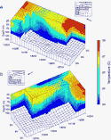
Click on thumbnail for full-sized image.

Fig. 25. Three-dimensional perspective plots of the vortex temperature and velocity viewed from the (a) southeast (30° south of east) and (b) northeast (30° north of east) at an inclination of 45°. Velocity vectors are projected onto the plane of each surface. Icons indicate projections of the cuts onto the horizontal plane (shaded) and vantage point (arrow) relative to the vortex flow.

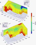
Click on thumbnail for full-sized image.

Fig. 26. Same as Fig. 25 but for salinity.

Click on thumbnail for full-sized image.

Fig. 27. Autocorrelation functions for: zonal velocity (solid lines), meridional velocity (dashed), and temperature (dash-dotted) for (a) drifters and (b) shipboard ADCP. (c) Temperature autocorrelation functions for the 2°N (solid) and 5°N (dashed) moorings. The integral timescales are taken to be one-half the lags at which the autocorrelation reaches zero.

*School of Ocean and Earth Sciences and Technology Contribution Number 4900.

⁺Current affiliation: Oceanographic Center, Nova Southeastern University, Dania Beach, Florida.

^#Additional affiliation: IFREMER, Plouzane, France.

REFERENCES

Baturin, N. G., and P. P. Niiler, 1997: Effects of instability waves in the mixed layer of the equatorial Pacific. J. Geophys. Res., 102, 27771–27793
Bingham, F. M., and R. Lukas, 1994: The southward intrusion of North Pacific Intermediate Water along the Mindanao coast. J. Phys. Oceanogr., 24, 141–154
Boyd, J. P., 1980: Equatorial solitary waves. Part I: Rossby solitons. J. Phys. Oceanogr., 10, 1699–1717
Bryden, H. L., and E. C. Brady,
1989: Eddy momentum and heat fluxes and their effects on the circulation
of the equatorial Pacific Ocean. J. Mar. Res., 47, 55–79
Busalacchi, A. J., M. J. McPhaden,
and J. Picaut, 1994: Variability in equatorial Pacific sea surface topography
during verification phase of the TOPEX/Poseidon mission. J. Geophys. Res., 99, 24725–24738
Carnevale, G. F., M. Briscolini,
R. C. Kloosterziel, and G. K. Vallis, 1997: Three-dimensionally perturbed
vortex tubes in a rotating flow. J. Fluid Mech., 341, 127–163
Chew, F., and M. H. Bushnell, 1990: The half-inertial flow in the eastern equatorial Pacific: A case study. J. Phys. Oceanogr., 20, 1124–1133
Cox, M. D., 1980: Generation and propagation of 30-day waves in a numerical model of the Pacific. J. Phys. Oceanogr., 10, 1168– 1186
Düing, W., P. Hisard, E. Katz, J.
Meincke, L. Miller, K. V. Moroshkin, G. Philander, A. A. Ribnikov, K. Voigt,
and R. Weisberg, 1975:Meanders and long waves in the equatorial Atlantic.
Nature, 257, 280–284
Firing, J., E. Firing, P. Flament, and R. Knox, 1994: Acoustic Doppler current profiler data from R/V Moana Wave
cruises MW9010 and MW9012. Tech. Rep. 93-05, SOEST, University of Hawaii,
Manoa, 114 pp. [Available from Satellite Oceanography Laboratory, SOEST,
University of Hawai’i at Manoa, Honolulu, HI 96822.]
Flament, P., and M. Sawyer, 1995:
Observations of the effect of rain temperature on the surface heat flux in
the intertropical convergence zone. J. Phys. Oceanogr., 25, 413–419
——, and L. Armi, 2000: The shear, convergence, and thermohaline structure of a front. J. Phys. Oceanogr., 30, 51–66
——, S. C. Kennan, R. Knox, P. Niiler,
and R. Bernstein, 1996: The three-dimensional structure of an upper ocean
vortex in the tropical Pacific. Nature, 382, 610–613
Flierl, G. R., 1981: Particle motions in large-amplitude wave fields. Geophys. Astrophys. Fluid Dyn., 18, 39–74
Halpern, D., R. A. Knox, and D.
S. Luther, 1988: Observation of 20-day period meridional current oscillations
in the upper ocean along the Pacific equator. J. Phys. Oceanogr., 18, 1514–1534
Hansen, D. V., and C. A. Paul, 1984: Genesis and effects of long waves in the equatorial Pacific. J. Geophys. Res., 89, 10431– 10440
——, and P.-M. Poulain, 1996: Quality control and interpolation of WOCE–TOGA drifter data. J. Atmos. Oceanic Technol., 13, 900–909
Harrison, D. E., 1996: Vertical velocity in the central tropical Pacific:A circulation model perspective for JGOFS. Deep-Sea Res., 43, 687–705
Hayes, S. P., L. J. Magnum, J. Picaut,
A. Sumi, and K. Takeuchi, 1991: TOGA TAO: A moored array for real-time measurements
in the tropical Pacific Ocean. Bull. Amer. Meteor. Soc., 72, 339– 347
Janowiak, J. E., and P. A. Arkin,
1991: Rainfall variations in the Tropics during 1986–89, as estimated from
observations of cloud-top temperature. J. Geophys. Res., 96, 3359–3373
Johnson, E. S., 1996: A convergent instability wave front in the central tropical Pacific. Deep-Sea Res., 43, 753–778
——, and D. S. Luther, 1994: Mean zonal momentum balance in the upper and central equatorial Pacific Ocean. J. Geophys. Res., 99, 7689–7705
Jourdan, D., P. Peterson, and C.
Gautier, 1997: Oceanic freshwater budget and transport as derived from satellite
radiometric data. J. Phys. Oceanogr., 27, 457–467
Kennan, S. C., 1997: Observations
of a tropical instability vortex. Ph.D. dissertation, SOEST, University of
Hawai’i at Manoa, 190 pp. [Available from Bell and Howell Information and
Learning (UMI), Ann Arbor, MI 48106; also available online at www.umi.com.]
Kloosterziel, R. C., and G. J. F. van Heijst, 1991: An experimental study of unstable barotropic vortices in a rotating fluid. J. Fluid Mech., 223, 1–24
Leetmaa, A., and R. L. Molinari, 1984: Two cross-equatorial sections at 110°W. J. Phys. Oceanogr., 14, 255–263
Legeckis, R., 1977: Long waves in the eastern equatorial Pacific Ocean: A view from a geostationary satellite. Science, 197, 1179–1181
——, 1986: A satellite time-series of sea surface temperature in the eastern equatorial Pacific Ocean. J. Geophys. Res., 91, 12879– 12886
——, W. Pichel, and G. Nesterczuk,
1983: Equatorial long waves in geostationary satellite observations and in
a multichannel sea-surface temperature analysis. Bull. Amer. Meteor. Soc., 64, 133– 139
Lindzen, R. S., 1988: Instability of plane parallel shear flow (toward a mechanistic picture of how it works). Pure Appl. Geophys., 126, 103–121
Lukas, R., 1987: Horizontal Reynolds stresses in the central equatorial Pacific. J. Geophys. Res., 92, 9453–9463
Luther, D. S., and E. S. Johnson,
1990: Eddy energetics in the upper equatorial Pacific during the Hawaii-to-Tahiti
Shuttle Experiment. J. Phys. Oceanogr., 20, 913–944
McClain, E. P., W. Pichel, and C. Walton, 1985: Comparative performance of AVHRR-based multichannel sea surface temperatures. J. Geophys. Res., 90, 11587–11601
McPhaden, M. J., 1995: The Tropical Atmosphere–Ocean array is completed. Bull. Amer. Meteor. Soc., 76, 739–741
——, 1996: Monthly period oscillations in the Pacific North Equatorial Countercurrent. J. Geophys. Res., 101, 6337–6359
Miller, L., D. R. Watts, and M. Wimbush, 1985: Oscillations of dynamic topography in the eastern equatorial Pacific. J. Phys. Oceanogr., 15, 1759–1770
Montgomery, R. B., and E. D. Stroup, 1962: Equatorial Waters and Currents at 150°W in July–August 1952. The Johns Hopkins Oceanographic Studies, No. 1, The Johns Hopkins University Press, 68 pp
Niiler, P. P., A. S. Sybrandy, K.
Bi, P.-M. Poulain, and D. Bitterman, 1995: Measurements of the water-following
capability of holey-sock and TRISTAR drifters. Deep-Sea Res., 42, 1951–1964
Perigaud, C., 1990: Sea level
oscillations observed with Geosat along the two shear fronts of the Pacific
North Equatorial Countercurrent. J. Geophys. Res., 95, 7239–7248
Philander, G., and Coauthors, 1985: Long waves in the equatorial Pacific Ocean. Eos, Trans. Amer. Geophys. Union, 66, 154
——, W. J. Hurlin, and R. C. Pacanowski,
1986: Properties of long equatorial waves in models of the seasonal cycle
in the tropical Atlantic and Pacific Oceans. J. Geophys. Res., 91, 14207– 14211
——, ——, and A. D. Seigel, 1987: Simulation of the seasonal cycle of the tropical Pacific Ocean. J. Phys. Oceanogr., 17, 1986– 2002
Pullen, P. E., R. L. Bernstein,
and D. Halpern, 1987: Equatorial long-wave characteristics determined from
satellite sea surface temperature and in situ data. J. Geophys. Res., 92, 742–748
Qiao, L., and R. H. Weisberg, 1995:
Tropical instability wave kinematics: Observations from the Tropical Instability
Wave Experiment. J. Geophys. Res., 100, 8677–8693
Rayleigh, L., 1916: On the dynamics of revolving fluids. Proc. Roy. Soc. London, 93A, 148–154
Sawyer, M., 1996: Convergence and
subduction at the North Equatorial Front. M.S. thesis, SOEST, University
of Hawai’i at Manoa, 92 pp. [Available from Bell and Howell Information and
——, P. Flament, and R. Knox, 1994: Hydrographic SeaSoar data from the R/V Moana Wave
cruises mw9010 and mw9012. Tech. Rep. 94-04, SOEST, University of Hawai’i
at Manoa, 101 pp. [Available from Satellite Oceanography Laboratory, SOEST,
Semtner, A. J., and B. M. Chervin, 1988: A simulation of the global ocean circulation with resolved eddies. J. Geophys. Res., 93, 15502–15522; 15767–15775
——, and ——, 1992: Ocean general circulation from a global eddy-resolving model. J. Geophys. Res., 97, 5493–5550
Trefois, C., P. Flament, R. Knox, and J. Firing, 1993: Hydrographic data from R/V Moana Wave
cruises MW9010 and MW9012. Tech. Rep. 93-01, SOEST, University of Hawai’i
at Manoa, 157 pp. [Available from Satellite Oceanography Laboratory, SOEST,
Tsuchiya, M., 1968: Upper Waters of the Intertropical Pacific Ocean. The Johns Hopkins Oceanographic Studies, No. 4, The Johns Hopkins University Press, 50 pp
——, 1991: Flow path of the Antarctic Intermediate Water in the western equatorial South Pacific Ocean. Deep-Sea Res., 38, S273–279
Vazquez, J., K. Perry, and K. Kilpatrick,
1998: NOAA/NASA AVHRR oceans pathfinder sea surface temperature data set
user’s reference manual. Tech. Rep. D-14070, Jet Propulsion Laboratory. [Available
online at podaac.jpl.nasa.gov./sst/sst_doc.html.]
Weare, B. C., P. T. Strub, and M. D. Samuel, 1981: Annual mean surface heat fluxes in the tropical Pacific Ocean. J. Phys. Oceanogr., 11, 705–717
Weisberg, R. H., J. C. Donovan,
and R. D. Cole, 1991: The Tropical Instability Wave Experiment (TIWE) equatorial
array: A report on data collected using subsurface moored acoustic Doppler
current profilers, May 1990–June 1991. Tech. Rep., University of South Florida,
106 pp. [Available from University of South Florida, St. Petersburg, FL 33701.]
Wilson, D., and A. Leetmaa, 1988: Acoustic Doppler current profiling in the equatorial Pacific in 1984. J. Phys. Oceanogr., 18, 1641– 1657
Wyrtki, K., and B. Kilonsky, 1984: Mean water and current structure during the Hawaii–Tahiti Shuttle Experiment. J. Phys. Oceanogr., 14, 242–254
Yoder, J. A., S. G. Ackleson, R. T. Barber, P. Flament, and W. M. Balch, 1994: A line in the sea. Nature, 371, 689–692