ABSTRACT

With the objective of measuring convergence directly to confirm previous observations of frontal subduction, a seaward upwelling jet off central California was studied using satellite infrared images, hydrographic sections, ship drift, and clusters of surface drifters. The cyclonic front of the jet was sharper than 1 km, resulting in a shear several times larger than f. A cross-frontal convergence of 7 cm s¹ over the width of the front (equivalent to 0.8f) was visible as a 20-m-wide accumulation of debris. The sharpness of the front lasted at least for a day. Away from the cyclonic front, the divergence of the flow was small and the shear was less than 0.6f. Thermohaline layers, originating at the front, were interleaving along isopycnals, suggesting water subduction. It is proposed that the asymetry between anticyclonic and cyclonic sides of the jet, and the strong convergence at the cyclonicfront, resulted from a frictionally driven ageostrophic secondary circulation superimposed on the geostrophic flow.

1. Introduction

The summertime mesoscale flow off central and northern California consists of large meanders of the California Current. The seaward branches of these meanders are narrow baroclinic jets, generally referred to as upwelling filaments, and they flow along the offshore boundary of the freshly upwelled coastal water. The cold temperature signature of these features was first observed by Bernstein et al. (1977) in satellite infrared images, and detailed in situ surveys of upwelling filaments were first made in 1981 and 1982 off Point Arena 39°N, 124°W (Flament et al. 1985 ; Kosro and Huyer 1986 ; Rienecker et al. 1985 ). The baroclinic jets have a width of 50 km, an offshore extension of up to 400 km, a maximum surface velocity of 80 cm s¹ decreasing with a depth scale of 150 m, and a total offshore transport of about 2·10⁶ m³ s¹. The surface layer processes associated with these jets are often asymmetric. Flament et al. (1985) found, at the anticyclonic boundary, a transition from cold to warm water spread over 20 km but, at the cyclonic boundary, a front sharper than 1 km where water subduction was observed. Similar observations were made subsequently during the 1987 Coastal Transition Zone experiment (Washburn et al. 1991 ; Huyer et al. 1991 ; Kosro et al. 1991 ; Dewey et al. 1991 ).

The specific objectives of the observations reported here were to study the velocity gradients associated with these fronts, resolving scales smaller than previously possible, and to observe the distribution of thermohaline fine structure. Satellite infrared images of sea surface temperature were used to guide the R/V Sproul to a filament off Point Sur (36°30N, 122°W), which was surveyed between 17 and 29 July 1985. The mesoscale structure of the filament, inferred from hydrographic stations, underway surface temperature and salinity, and drifters tracks, is presented in section 2. Measurements of velocity gradients and frontal convergence, using surface drifters deployed in clusters and ship drift, are presented in section 3. The fine structure observed in the hydrographic stations and tow-yo CTD sections are described in section 4. These observations are summarized and interpreted in terms of surface layer processes in section 5. The technique for measuring velocity gradients using clusters of drifters is discussed in the appendix. Details about the other instruments and data processing can be found in the appendix to Flament et al. (1985) .

2. Mesoscale structure of the filament

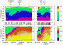
Two 24-h sequences of cloud-free satellite infrared images from the National Oceanic and Atmospheric Administration (NOAA) polar orbiting satellites were acquired, before the cruise on 8 and 9 July and after the cruise on 5 and 6 August. Marine stratus covered the area during most of the cruise, yielding only a single usable image on 24 July. The images of 0300 UTC 9 July, 0300 UTC 24 July, and 1000 UTC 5 August are shown in Fig. 1 . A cold filament was rooted near 35°30N, 122°W, meandering toward the southwest. Near 34°30N, 123°W, it turned sharply to the southeast, following a persistent large-scale zonal front. Its maximum offshore extension was 250 km. Small thermal features with scales of 1 to 5 km, passively advected by the mesoscale flow, were used to estimate surface velocities from the sequences of images. The cold filament was the surface expression of a jet flowing offshore, with speeds reaching at least 50 cm s¹.

The schedule of the ship survey is shown in Fig. 2 . The wind was upwelling-favorable during most of the survey, except during two short relaxation events on 19 and 26 July. The positions of the CTD stations relative to the boundaries of the filament on 24 July 1985 are shown in Fig. 3 . The survey started on 20 July with a section to locate the jet, then proceeded northward until 26 July, the section being repeated four times to detect temporal variations of the flow.

Mixed layer drifters were deployed during the survey, either individually or in clusters. Surface velocities were inferred from successive positions of these drifters (Fig. 3 ); the median speed for the drifters deployed in the jet was 51 cm s¹, consistent with the speed inferred from the sequences of satellite images (Fig. 1 ).

Surface temperature, salinity, geopotential anomaly referenced to 500 dbar, and a contour plot of geostrophic velocity along the section made on 20 July are displayed in Fig. 4 . Given the consistently southward direction followed by the drifters released in the jet near the section, geostrophic velocity was computed assuming a southward flow. Centripetal accelerations, estimated from the curvature of the filament, were less than 20% of the Coriolis accelerations and were neglected. The width of the jet was 30 km and its geostrophic transport referenced to 500 dbar was 2.0·10⁶ m³ s¹. East of the jet, there was a weak northward geostrophic flow of 8 cm s¹. The flow was strongly surface intensified;the geostrophic velocity referenced to 500 dbar exceeded 90 cm s¹ at the surface, but decreased to less than 20 cm s¹ at 100-m depth (Fig. 5 ); for reference, the velocity profile observed by Flament et al. (1985) is also shown in Fig. 5 (dashed). The large magnitude of surface velocity was confirmed by a drifter, which, launched near the axis of the jet, averaged 84 cm s¹ southward over 6 hours.

This filament and the filament repeatedly surveyed off Point Arena (Flament et al. 1985 ; Kosro and Huyer 1986 ; Rienecker et al. 1985 ), appear to have very similar structures. Both corresponded to shallow baroclinic jets transporting offshore a few Sverdrups of cold surface water, bounded by warm and salty water on the cyclonic (southeastern side) and warm and fresher water on the anticyclonic (northwestern) side. Both were surface intensified, and both were associated with a shoreward flow on their cyclonic side.

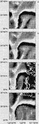
Surface isotherms appear to converge toward the cyclonic front near 35°20N, 122°10W in the sequence of images from 9 July, enhanced and enlarged in Fig. 6 . The distance between the front and a mushroom-shaped patch of cold water to the east, decreased from 14 to 8 km after 12 hours and to 5 km after 24 hours. Assuming the isotherms spacing to decrease as s = s₀e^t, s being a cross-isotherm coordinate, a rough estimate of the convergence rate is 1.2·10⁵ s¹ f/7 (all velocity gradients will be given in units of f = 8.6×10⁵ s¹, the planetary vorticity at this latitude). A cross-isotherm convergence toward the cyclonic boundary was also inferred from satellite images by Flament et al. (1985) .

A longitude/time contour of geopotential anomaly of the surface referenced to 500 dbar along the repeated section reveals a westward translation of the structure (Fig. 7 ). Multiple linear regression of geopotential anomaly versus time and longitude yields a translation speed to the west of 4.3 ± 0.7 cm s¹ (one standard deviation). This translation was also observed in the satellite images: between 9 July and 5 August, the position at which the filament crossed the 2000-m isobath, chosen to represent the shelf break, moved about 75 km to the northwest, an average of 3.5 cm s¹ (Fig. 1 ).

3. Velocity gradients

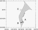
Three clusters of nine drifters each were deployed to directly measure the velocity gradients at a scale of a few kilometers. Details of the experimental technique and the estimation of the flow parameters are discussed in the appendix. The positions of the clusters relative to the boundaries of the cold filament observed in the image of 24 July are shown in Fig. 8 . Cluster A spanned the sharp cyclonic front, cluster B was deployed near the axis of the cold filament, and cluster C was deployed farther west on the anticyclonic side of the jet. The initial grid spacing, the time and coordinates of the deployments, and the tracking period of each cluster are given in Table 1 . As explained in the appendix, large horizontal strain limited the tracking period of the clusters to a few hours, less than the tidal and inertial periods.

The trajectories of the drifters in cluster A, tracked for about 8 hours with an initial grid spacing of 2 km, are shown in Fig. 9 . The flow was discontinuous at the spacing of the drifters; three drifters moved rapidly southward in the jet, whereas most of the drifters east of the jet moved slowly northwestward. The flow parameters, assuming slablike motions on either side of the front, are listed in Table 1 . The cyclonic shear _x across the front was larger than /x = 2.9f and there was a cross-frontal convergence _xu stronger than u/x = 0.45f. These are lower bounds because the width of the front was considerably less than the spacing of the drifters. Surface salinity sampled while tracking this cluster is shown in Fig. 9b , with light gray shades representing the high salinity warm water. The southward jet corresponded to a transition from low salinity water (S = 32.9 psu) in the filament to high salinity water (S = 33.4 psu) to the east. Surface temperature variations were masked by intense diurnal warming (Flament et al. 1994 ) and were therefore difficult to relate to the velocity front.

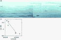
A 20 m wide accumulation of debris, consisting of seaweeds such as Macrocystis pyrifera, ship refuse, sonobuoy containers, and bales of Canabis sativa, was found along the sharp front. A photograph of the accumulation of debris is shown in Fig. 10 . The drifters launched east of the jet were retrieved in this debris line, which extended straight from horizon to horizon at 190° heading. The line was crossed repeatedly for several days (although its position was only recorded on 26 and 27 July), and it migrated westward at 6 cm s¹ (Fig. 10 , inset) following the translation of the jet (Fig. 9b is therefore not a truly synoptic view of the surface salinity field). No other accumulation lines were observed during the cruise.

For the purpose of detecting possible variations of water velocity across the debris line, the ship was slowed down to a constant speed of 1.3 m s¹ and steered on a constant gyrocompass heading orthogonal to the line. The ship track crossing the line and entering the southward jet is shown in Fig. 11 . Surface temperature, salinity, and density during the transect, also shown in Fig. 11 , confirm that the debris line coincided with the eastern boundary of the filament.

Surface currents, derived from the difference between velocity over ground using LORAN-C and velocity over water using the electromagnetic log and the gyrocompass, are given in Table 1 . The alongfront flow varied from 2 cm s¹ east of the line to 64 cm s¹ in the jet, over a region 1 km wide starting at 122°30.5W that ended at 122°31.5W. The 1-km scale of the transition suggests a horizontal shear larger than 7.5f and a cross-frontal convergence stronger than 0.8f. Closer examination of the track indicates that the transition may have been concentrated over two very narrow regions barely resolved by the 80-m sampling of the LORAN-C, implying even larger shear and converge rate. Unfortunately, for all other crossings of the jet, the ship was steered with the LORAN-C navigator on a constant track over ground, and gyrocompass heading was not recorded. These other crossings cannot be used to infer subtle variations of water velocity through the drift of the ship.

In contrast to the sharp front spanned by cluster A, the velocity field appeared continuous at clusters B and C, varying over spatial scales larger than the span of the clusters and over temporal scales longer than their tracking periods. The flow u(r, t) can therefore be approximated by a linearized Taylor series in the vicinity of some reference point r₀:

u(r) = u₀ + (r r₀), (1)

It is customary to decompose a velocity gradient tensor into an antisymmetrical part = u u representing vorticity and a symmetrical part = u + u representing irrotational deformation, which can be further decomposed into an isotropic divergence Tr() and a nondivergent strain, = Tr()/2 (cf. Batchelor 1967 , p. 79). The eigenvectors of represent the principal axes of expansion and contraction. Such decomposition of relative motion, of course, is not unique. Since the jet is approximately a parallel shear flow, in which the mean velocity is an order of magnitude larger than the velocity difference across the clusters, it is also useful to decompose u into a pure shear parallel to the mean flow, an isotropic divergence, and a residual pure strain or confluence, as given in Table 1 .

To interpret Table 1 and summarize this section, the clusters and the ship crossing provided direct measurements of the variations of horizontal shear across the filament: from 0.6f on the anticyclonic side (A), to 1.2f near the axis (B), and to several times f at the cyclonic front (more than 2.9f from cluster A and more than 7.5f from the ship drift). These astounding magnitudes of cyclonic vorticity can be compared with the much smaller background vorticity of 0.05f inferred 25 km to the southeast of a filament rooted at the same location a year earlier (see appendix). A cross-frontal convergence stronger than 0.8f was observed at the cyclonic front, causing the accumulation of debris observed repeatedly over several days. The alongfront gradients and thus total divergence and residual strain could not be measured directly there, the cluster being too rapidly elongated along the front to provide reliable estimates of u.

There was a small isotropic divergence of 0.3f near the axis (B), suggesting that the cold anomaly may have been partially maintained by local upwelling. There was also a small isotropic convergence of 0.3f on the anticyclonic side (C). A significant residual strain of 0.6f was observed near the axis and on the anticyclonic side, with the diverging principal direction of the strain oriented nearly parallel to the mean flow within sampling errors at both locations, suggesting that the narrowness of the filament may have been partially maintained by such confluence.

4. Thermohaline structure

In this section, CTD stations from the hydrographic survey along with tow-yo sections at fine horizontal resolution will be used to discuss the thermohaline structure in the neighborhood of the upwelling filament. It will be shown that mixing at and beneath the jet was primarily along isopycnals, with sharp subsurface fronts.

The hydrographic stations can be grouped into four types (Fig. 14 ). For stations east of the filament (type“East”), salinity, from 33.7 at the surface, varies little down to the 26.0 isopycnal at about 75-m depth. Beneath, salinity gradually increases to 34 as the temperature further decreases to 6°C through the upper thermocline. In contrast, for stations to the west of the filament (types “West” and “Far West”), salinity first decreases from 33 at the surface to a minimum of 32.8 on the 25.2 isopycnal at 50-m depth, then rapidly increases to 33.7 on the 26.0 isopycnal, and finally follows at greater depths the same T–S relationship as stations to the east. The stations immediately to the west of the front (type “West”) differ slightly between the 25.3 and 26.0 isopycnals from stations farther to the west (type “Far West”), possibly reflecting a different upstream origin of this deeper water, but the overall structure of the water column is similar.

Profiles characterized by multiple thermohaline inversions are found in the vicinity of the cyclonic front, suggesting strong interleaving at the boundary between the two extreme water column types (shown as“Mixed” in Fig. 14c ). The vertical scale of the interleaving is typically 10 to 20 m, with little spatial correlation between neighboring stations.

To gain more insight into the relationship between the thermohaline inversions and the front, two CTD tow-yo sections were conducted across the filament, one near where the clusters were deployed, the other about 50 km upstream, closer to the root (Fig. 15 ). The temperature and salinity fields are shown in Fig. 16 , with the isopycnals overlaid.

Both sections reveal a strong subsurface front spanning the 25.0 to 26.0 isopycnals, separating warmer and more saline waters to the east from colder and fresher waters to the west. Thermohaline intrusions are observed along isopycnals, interleaving away from the subsurface front at 122°45W, mostly in the northern section. On any isopycnal, the transition between the two water column types is abrupt, barely resolved by the 500 m horizontal resolution of the tow-yo.

Above the 25.0 isopycnal, the T–S relationships on both sides of the front are affected by intense diurnal surface warming, a result of the slack winds observed during the tow-yos on 25 to 27 July (Fig. 2 ). These warming events are seen as thin 13° to 16°C layers, extending from the surface to a sharp thermocline at 10 m depth. There is no evidence of a well-mixed surface layer, and no corresponding halocline. The warm surface layers appear to be interrupted near the axis of the jet, where colder water at 12.5°C outcrops, possibly confirming the divergence sampled by cluster B in this part of the jet. Although the surface warming masks the temperature front, the convergence is nevertheless observable at the surface, as evidenced by the debris line shown in Fig. 10 .

Our interpretation of the overall thermohaline structure of the filament is summarized by Fig. 17 , showing the median T–S profile of each water column type observed. Slicing off an 20 m deep surface layer affected by diurnal warming, the remaining T–S configuration is reminiscent of that observed by Flament et al. (1985) off northern California. To the east of the filament, warm saline water is found on the 25.7 isopycnal and below. As one progresses westward at constant density, this layer becomes deeper and is capped by a layer of colder and less saline water. However, the horizontal extent of the subducted layer—limited by the subsurface front—is much shorter than observed by Flament et al. (1985) , that is, a few kilometers versus a few tens of kilometers. The large low salinity inversion found at depth 80 to 120 m farther west appears to originate at the root of the filament nearshore, rather than result from a cross-frontal subduction.

5. Summary and discussion

Through a small-scale sampling of the velocity structure of a seaward filament rooted off central California, we have inferred that 1) the cyclonic front of the filament was sharper than 1 km, resulting in a horizontal shear that reached several times f; 2) elsewhere, the shear was less than 0.6f; 3) a cross-frontal convergence 7 cm s¹ over less than 1 km (larger than 0.8f) was visible as a 20 m wide accumulation of debris coinciding with the cyclonic front; 4) elsewhere, the divergence was small; and (5) the sharp front persisted at least for a day—a period much longer than the timescale corresponding to the vorticity (i.e., 2/7.5f = 2.7 h). The asymmetry between the cyclonic and anticyclonic sides of the jet and the very large cyclonic shears are consistent with the findings of Flament et al. (1985) , but has now been observed at higher resolution, with the shear and convergence rates being measured directly with surface drifters, not just indirectly from satellite images.

Very sharp convergent shear fronts associated with upwelling filaments have been reported by others. Aside from Sheres et al. (1985) , who inferred a shear of 10f from swell refraction seen in an image taken from aircraft, Moum et al. (1990) found a convergent slick, observed as a thickening of the surface microlayer, coinciding almost exactly with the temperature front of a filament off Point Arena. Very similar to our observations were the measurements of Sanford et al. (1988) . Using a towed geomagnetic electro-kinetograph, they measured relative vorticities reaching 6.5f at the southern boundary of a filament off Cape Mendocino, but only 0.5 to 1f near the northern boundary. The velocity signature was entirely baroclinic with no detectable barotropic shear. There is therefore a consistent set of observations suggesting that sharp convergent shear fronts may be a general feature of upwelling filaments.

The subsurface temperature and salinity fields reflected this cross-frontal circulation. Although details of the thermohaline structure depend on many factors, including the specific T–S relationships of the upstream source waters and the effects along the offshore advection path of wind stress (the case of Flament et al. 1985 ) or heat flux (this experiment) on the surface layer, isopycnal interleaving suggestive of subducted layers, and sharp O(100 m) thermohaline fronts, have been consistently observed.

Mechanisms that may force the observed convergences fall in two categories: those resulting from cross-frontal variation of the wind-driven Ekman transport, and those resulting strictly from oceanic processes. A straight two-dimensional jet flowing westward (U(y) < 0) will be assumed, y being the cross-front coordinate.

For a slablike mixed layer, the cross-frontal depth-averaged generalized Ekman velocity is

, U,

1. A change of the drag coefficient C_D, hence of , results from variations of the air–sea temperature difference (Businger and Shaw 1984 ; Hanson 1987 ). For a column of air initially in thermal equilibrium with water, reaching a 1.5°C front, C_D varies by 25% at 2 m s¹ and 15% at 5 m s¹ (Smith 1988 ). This effect decreases rapidly as the wind speed increases. In the Northern Hemisphere, Ekman convergence occurs where colder water is to the right of the wind.

2. Since the local vorticity _yU varies across the jet, the magnitude of V_e decreases on the cyclonic side and is enhanced on the anticyclonic side. Ekman convergence results when _xyyU > 0, or along the axis for a westerly wind blowing against a westward jet (Niiler 1969 ; cf. also Stern 1975 ). For shear variations of order f, order 1 variations of the Ekman transport result, consistent with the convergence rates observed.

3. Variations of H may result from different deepening histories of the mixed layers on either side of a front, having been advected from different origins, and their deepening having been modulated by the varying horizontal shear (Klein and LeSaos 1986 ). Ekman convergence is induced where _xyH < 0.

Although these wind-driven processes are certainly able to force convergences, they cannot alone explain the consistent asymmetry of the filaments: sharp fronts have always been observed on the cyclonic side of the offhsore-flowing jets, yet a change of sign of in (2) would permute convergent and divergent regions. Could an oceanic process independent of the wind be invoked?

The convergence may indeed be a secondary frictional flow V_f induced by the alongfront geostrophic flow U_g:

fV_f = ²_zzU_g, (3)

z/z₀

1

Clearly, several processes may contribute to force the convergence, some playing a dominant role in low wind conditions (this paper; Moum et al. 1990 ) and others in high wind conditions (Flament et al. 1985 ; Sheres et al. 1985 ; Sanford et al. 1988 ). Although the data presently available are not sufficient to single any out, the frictional effect on the mean flow has the appeal of universality. It yields an intriguingly simple scale for the width of surface and subsurface fronts in advective–diffusive balance. The equilibrium width of such fronts is (Thorpe 1983 )

l = 2(_h/_yV)^1/2. (5)

l = 2(_h/)^1/2Ro^1/2z₀,

Acknowledgments. Precise maneuvers by L. Zimm, master of the R/V E. B. Scripps in 1984, and by T. Beattie, master of the R/V R. G. Sproul in 1985, made tracking the drifters possible. D. Chester, L. Christel, M. Crawford, R. Olsen, S. Taylor, C. Trefois, and S. Yamasaki helped with the operations at sea. M. Sawyer prepared the figures using the plotting package gri by D. Kelley. R. Hansen, S. Laurent, and S. Laurent helped clarify the cluster bootstrapping procedure. R. Hall gave insightful comments on the effects of friction. This work was supported by the Office of Naval Research (Contracts N000014-80-C-0440, N00014-87-K-007, N00014-96-1-0411).

We present the technique used for measuring the surface velocity gradient tensor u at a scale of a few kilometers, using clusters of drifting buoys tracked for a few hours. Measurements of u at the surface are not new: examples based on triads of drifters can be found in Reed (1971) , Chew and Berberian (1971) , Molinari and Kirwan (1975) , Kirwan (1975) , and more recently in Niiler et al. (1989) . Here, we used a larger number of drifters, allowing better estimation of standard errors.

The subsurface drifter introduced by Davis (1985) , minimizing the rectification of wave forces and the wind drag, was used. It consists of a radio beacon connected to a drogue by a polyamide line. A flashing light was attached to the antenna to assist in tracking. In a preliminary test, large vertical shears caused the original dihedral drogues to kite and the line to be pulled up to 60° from the vertical (i.e., the drogue was subject to a lift force instead of a pure drag). A fifth sail was therefore added to prevent lift, closing the lower face of the dihedral angle.

Drifters were deployed in clusters of nine on a 3 by 3 square grid with a grid spacing of 1 to 4 km and tracked while the seeded parcel of water was advected and deformed by the mesoscale flow. They were tracked by homing the ship successively to each drifter, resulting in a set of nonsynchronous positions every 2 to 5 hours. A LORAN-C receiver was used for navigation. Random position errors were estimated to be 70 m in latitude and 100 m in longitude.

The following notations will be used: r_ip is the ith position on drifter p taken at time t_ip, r_ip = r_i+1p r_ip is the displacement of drifter p during the interval t_ip = t_i+1p t_ip, and _ip = (r_ip + r_i+1p)/2 is the mean position of the drifter during that interval.

Away from fronts, the mesoscale velocity field u(r,t) is assumed to vary over a temporal scale longer than the inertial period and over a spatial scale larger than the internal radius of deformation, typically 30 km for the midlatitude eastern Pacific (Emery et al. 1984 ). The clusters were much smaller, and were tracked for an inertial period or less. The value u(r) can therefore be approximated by a Taylor series limited to first order:

u(r) = u₀ + (r r₀),

d_tr = u₀ + (r r₀). (A1)

We used instead a simple linear pseudo Eulerian model based on a centered first difference approximation of (A1):

r_ip = u₀t_ip + (_ip r₀)t_ip + r_ip, (A2)

Minimization of the residual variance {|r_ip|²} yields normal equations for u₀ and = [a]:

The expression for the variance of the parameters of a minimum mean square error model yields (cf. Meyer 1975 ):

ip

a

Alternately, standard errors on u₀ and can be obtained by a stochastic procedure, in which the configuration of the sampling cluster is varied randomly while statistics of the estimated parameters are collected (a so-called “bootstrap,” Efron and Gong 1983 ; see, also, D’Asaro 1985 ; Kunze and Sanford 1986 ). Randomly resampled clusters were constructed by drawing with replacement n × n drifters out of the original cluster, allowing duplications and omissions (limited to two to prevent the generation of singular clusters). The parameters were then estimated from the original positions on each resampled cluster, and the probability density functions and standard deviations of the parameters computed.

The technique was tested in 1984. Satellite thermal infrared images were used to guide the ship away from large horizontal velocity gradients. The cluster was deployed in an isothermal region, 25 km to the southeast of the cold filament originating near Point Sur (36°30N, 122°W), in water 3000 m deep. Hydrographic stations showed a 20-m-deep mixed layer, which remained at a constant temperature of 16°C while the cluster was tracked. The drifters were drogued at half the mixed layer depth.

The spacing of the drifters was 4.5 km; a set of positions was obtained every 5 h for about 24 h (Fig. A1 ). The drifters moved westward at a nearly uniform speed of 24 cm s¹. The estimated flow parameters are given in Table A1 , with standard errors determined from 10⁴ bootstrap realizations. The standard error computed from (A2) is 2.4·10⁶ s¹, similar to the bootstrap errors. The velocity gradient corresponded to a weak but significant positive vorticity (a₂₁ a₁₂) = 4.3×10⁶ s¹ f/20. Figure A2 shows the trajectories in the absolute frame of reference, and in the frame of reference translating with the mean flow u₀. The weak vorticity is noticeable (cf. drifters 8 with 4, or 6 with 2).

The rms residual displacement {|r_ip|²}^1/2, unexplained by the model, is about 750 m for each component, larger than the LORAN-C position error. Several processes may contribute to these residuals. The model of Pollard and Millard (1970) predicts wind-driven inertial oscillations of 2 cm s¹, corresponding to a gyration radius of 240 m. Typical amplitudes for the semidiurnal tide and the diurnal tide off California are 4 and 1 cm s¹ (Noble et al. 1986 ; Munk et al. 1970 ), corresponding to displacements of 280 and 140 m. The rms horizontal displacement due to the internal wave continuum, modeled by the canonical GM-79 spectrum extrapolated to the surface (Munk et al. 1981 ), is 420 m for each component. Incoherently adding these variances gives rms residuals of 520 m for each component, in fair agreement with the observed residuals. Drifters may also be entrained in Langmuir cells, often associated with down-wind jets (Weller et al. 1985 ), further increasing the residuals.

Weak temporal modulations are in fact present in the residuals. Longitudinal and transverse correlation functions are defined as

This test showed that, in a region with negligible gradients, incompletely sampled tidal, near-inertial, and internal waves resulted in a standard error of 2×10⁶ s¹ f/40. The error would increase for stronger inertial oscillations, unless the sampling scheme can resolve them. The estimation error cannot be easily decreased by increasing the number of drifters or the tracking period, since the assumption of a scale separation between residual motions and mesoscale flow constrains the cluster size nL to be smaller than the internal radius of deformation, and since the assumption that the mesoscale flow is steady forbids making the tracking period mT much larger than 1/f. As we found in section 3, this constraint is most severe in regions subject to large horizontal straining: after a time = ¹, clusters are too elongated to provide reliable estimates of u

Dewey, R. K., J. N. Moum, C. A. Paulson, D. R. Caldwell, and S. D. Pierce, 1991: Structure and dynamics of a coastal filament. J. Geophys. Res., 96, 14885–14908.

Flament, P., L. Armi, and L. Washburn, 1985: The evolving structure of an upwelling filament. J. Geophys. Res., 90, 11765–11778.

Huyer, A., and Coauthors, 1991: Currents and water masses of the coastal transition zone of northern California. J. Geophys. Res., 96, 14809–14832.

——, ——, and Coauthors, 1991: The structure of the transition zone between coastal waters and the open ocean off northern California, winter and spring 1987. J. Geophys. Res., 96, 14707–14730.

Smith, S. D., 1988: Coefficients for sea surface wind stress, heat flux and wind profile as a function of wind speed and temperature. J. Geophys. Res., 93, 15467–15472.

Washburn, L., D., Kadko, B. H. Jones, T. Hayward, P. M. Kosro, T. P. Santon, S. Ramp, and T. J. Cowles, 1991: Water mass subduction and the transport of phytoplankton in a coastal upwelling system. J. Geophys. Res., 96, 14927–14946.

Click on thumbnail for full-sized image.

Fig. 1. Thermal infrared images from the NOAA polar orbiting satellites: (a) 0300 UTC 9 Jul, (b) 0300 UTC 24 Jul, (c) 1000 UTC 5 Aug. Light gray shades correspond to cold water. Surface velocities obtained by following thermal features over an 24-h period are overlaid on (a) and (c). No sequence exists for (b). The 2000-m isobath is shown by a dashed line.

Click on thumbnail for full-sized image.

Fig. 2. Schedule of the experiment, showing the times of cloudless satellite images, of underway sampling of surface temperature and salinity, of the hydrographic stations, of the tow-yo sections, of the drifters fixes, of the sightings of the debris line, and of the ship drift study. A time series of the alongshore (southeastward) component of the wind from the log of the R/V Sproul is also shown.

Click on thumbnail for full-sized image.

Fig. 3. Velocity vectors from individual drifters deployments and actual positions of the hydrographic stations. For reference, the boundaries of the cold filament on 24 July are shown stippled. The section along the dashed line was repeated four times during the cruise. The stations shown in Fig. 14 are marked with a star. The positions of the drifters clusters and of the tow-yo sections are shown in Fig. 8 and Fig. 15 .

Click on thumbnail for full-sized image.

Fig. 4. Hydrographic section along the NW–SE line shown in Fig. 3 , using stations taken on 20 and 21 July: (a) surface temperature, (b) surface salinity, (c) surface geopotential anomaly, (d) surface geostrophic velocity, (e) contours of geostrophic velocity at 0.1 m s¹ intervals. (c), (d), (e) are referenced to 500 dbar.

Click on thumbnail for full-sized image.

Fig. 5. Profiles of geostrophic velocity referenced to 500 dbar. Solid: between two stations spaced 7 km apart near the axis of the jet. Dashed: between two stations spaced 8 km apart near the axis of the jet rooted near Point Arena in 1982 (from Flament et al. 1985 ).

Click on thumbnail for full-sized image.

Fig. 6. Sequence of images showing a region of cross-isotherm convergence near the dotted line: (a) 2200 UTC 8 Jul, (b) 0300 UTC 9 Jul (also shown in Fig. 1 ), (c) 1500 UTC 9 Jul, (d) 0300 UTC 10 Jul. These images were enlarged and enhanced by a high-pass filter to emphasize small thermal features.

Click on thumbnail for full-sized image.

Fig. 7. Time/longitude contour plot of geopotential anomaly along repeated section, showing northwestward translation of the field.

Click on thumbnail for full-sized image.

Fig. 8. Positions of the clusters with respect to the boundaries of the cold filament observed in the image of 24 July, shown stippled. The positions have been extrapolated to the time of the image to correct for the translation speed inferred from Fig. 7 . The ship track used to estimate ship drift is also shown.

Click on thumbnail for full-sized image.

Fig. 9. (a) Linearly interpolated drifters trajectories for cluster A, deployed starting 1700 UTC 26 Jul (cf. Fig. 2 ). The distances between successive dashes in the trajectories correspond to ½ hour. The launch positions are shown as dots and the recorded positions are shown as stars. The approximate position of the debris line relative to the cluster is shown by a thick line. (b) Map of surface salinity sampled while tracking this cluster, with dark gray shades representing low salinity cold water. The north–south salinity front corresponding to the eastern boundary of the jet is seen. The origin of the coordinates is at 35°40N, 122°28W.

Click on thumbnail for full-sized image.

Fig. 10. A panorama of photographs of the accumulation of debris taken 1530 UTC 27 Jul, viewing toward the southwest (left), west (center), and northwest (right). The inset shows longitude of the debris line as a function of time.

Click on thumbnail for full-sized image.

Fig. 11. Ship track crossing the convergence zone from east to west at 1.3 m s¹, starting 0630 UTC 27 Jul. LORAN-C positions are shown at 1-min intervals (100 m). The latitude scale has been exaggerated by a factor of 3 to show the southward drift of the ship entering the jet. The position of the debris line is shown by a dashed line. Surface density, temperature, and salinity during the crossings are shown in the lower panels.

Click on thumbnail for full-sized image.

Fig. 12. (a) Linearly interpolated drifters trajectories for cluster B, deployed starting 0930 UTC 27 Jul. The drifters are numbered at their launch position and the recorded positions are shown as stars. The origin of the coordinates is at 35°37N, 122°31W. (b) Trajectories in the frame of reference translating with the mean flow. The distance between successive dashes in the trajectories corresponds to interpolated intervals of ½ hour.

Click on thumbnail for full-sized image.

Fig. 13. Same as Fig. 12 but for cluster C, deployed starting 1930 UTC 24 Jul. The origin of the coordinates is at 35°56N, 122°32W.

Click on thumbnail for full-sized image.

Fig. 14. Aggregate T–S diagrams for the four water column types identified: (a) “Far West” of the filament, (b) “West” of the front, (c) “Mixed” mixing region near the front, (d) “East” of the front. The top panel shows the position of the stations used for each type. The bottom panel shows vertical profiles of temperature and salinity for a typical station in each type, marked by a star in the top panel (see also Figs. 3 and 15 for the location of these stations).

Click on thumbnail for full-sized image.

Fig. 15. Positions of the tow-yo sections and of the four CTD stations shown in Fig. 14 with respect to the boundaries of the cold filament observed in the image of 24 Jul. The positions of the sections have been extrapolated to the time of the image to correct for the translation speed inferred from Fig. 7 .

Click on thumbnail for full-sized image.

Fig. 16. Tow-yo sections of temperature (top) and salinity (bottom) vs pressure across the filament. Left panels: tow-yo I; right panels: tow-yo II. The depth/distance path of the undulating CTD is shown above each section. The isopycnals are overlaid.

Click on thumbnail for full-sized image.

Fig. 17. Summary of the four basic water column types, shown as the isopycnal-averaged T–S diagram of each type (see text).

Click on thumbnail for full-sized image.

Fig. A1. Drifters tracking schedule. The origin of time is set at the start of the deployment, 1820 UTC 11 Aug.

Click on thumbnail for full-sized image.

Fig. A2. (a) Linearly interpolated trajectories, dashed every hour. The deployment configuration of the cluster is outlined. The origin of coordinates is set at 36°10N, 122°36W. (b) Residual trajectories dashed every hour, after removing the mean translation. The start of each track is marked by a star. The radii of the concentric circles represent the 750-m rms residual displacement and the 100-m rms LORAN-C error.

Click on thumbnail for full-sized image.

Fig. A3. (a) Temporal longitudinal coherence function C_L(r < 6 km, t); (b) temporal transverse coherence function C_T(r < 6 km, t). Here, f indicates the inertial period.

*School of Ocean and Earth Sciences and Technology, University of Hawaii Contribution Number 4898.

Table 1. Flow parameters.

Table A1. Flow parameters.

REFERENCES

Batchelor, G. K., 1967: Fluid Dynamics. Cambridge University Press 615 pp.
Bernstein, R. L., L. Breaker, and R. Whritner, 1977: California current eddy formation. Science, 195, 353–359.
Businger, J. A., and W. J. Shaw,
1984: The response of the marine boundary layer to mesoscale variations in
sea-surface temperature. Dyn. Atmos. Oceans, 8, 267–281.
Chew, F., and G. A. Berberian, 1971: A determination of horizontal divergence in the Gulf Stream off Cape Lookout. J. Phys. Oceanogr., 1, 39–44.
D’Asaro, E. A., 1985: Upper ocean
temperature structure, inertial currents and Richardson numbers observed
during strong meteorological forcing. J. Phys. Oceanogr., 15, 943–962.
Davis, R. E., 1985: Drifter observations of coastal surface currents during CODE: the method and descriptive view. J. Geophys. Res., 90, 4741–4755.